|
Normal Probability Distribution
|
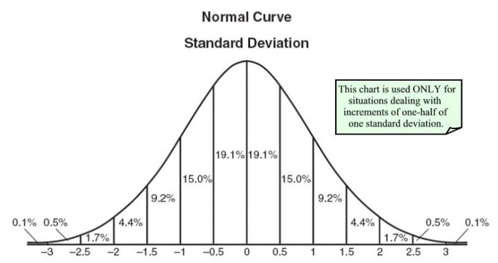
Chart prepared by the NY
State Education Department |
|
A chart, such as that seen above, is often used
when dealing with normal distribution questions. Understand
that this chart shows only percentages that correspond to
subdivisions up to one-half of one standard deviation.
Percentages for other subdivisions require a statistical
mathematical table or a graphing calculator.
(See example 4) |
|
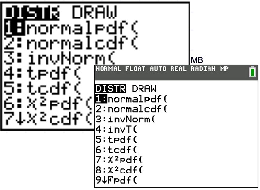
The Normal Probability Distribution menu for the
TI-84+ is found under DISTR (2nd
VARS).
NOTE:
A mean of zero and a standard
deviation of one are considered to be the default values for a
normal distribution on the calculator, if you choose not to set
these values. |
|
|
The Normal Distribution
functions:
#1: normalpdf pdf = Probability Density Function
This function
returns the probability of a single value of the random variable x. Use this to graph a normal curve. Using
this function returns the y-coordinates of the normal
curve.
Syntax: normalpdf (x, mean, standard
deviation)
#2: normalcdf
cdf = Cumulative
Distribution Function
This function returns the
cumulative probability from zero up to some input value of the
random variable x.
Technically, it returns the percentage of area under a
continuous distribution curve from negative infinity to the x.
You can, however, set the lower bound.
Syntax:
normalcdf (lower bound, upper bound,
mean, standard deviation)
#3: invNorm( inv = Inverse Normal Probability
Distribution Function
This function returns the x-value given the probability region
to the left of the x-value.
(0 < area < 1 must be
true.) The inverse normal probability distribution function
will find the precise value at a given percent based upon the
mean and standard deviation.
Syntax: invNorm (probability, mean, standard
deviation)
|
Example 1:
Given a normal distribution of values for which the mean is 70 and the
standard deviation is 4.5. Find:
a) the probability that a value is between 65 and 80,
inclusive.
b) the probability that a value is greater than or equal to
75.
c) the probability that a value is less than 62.
d) the 90th percentile for this distribution.
(answers will be rounded to the nearest thousandth) |
|
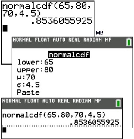
1a:
Find the probability that a value is between 65 and 80,
inclusive. (This is accomplished by finding the
probability of the cumulative interval from 65 to 80.)
Syntax:
normalcdf(lower bound, upper bound,
mean, standard deviation)
Answer:
The probability is 85.361%.
(The "PASTE" command simply means that the values that you
typed after the template prompts will be "pasted" into the
normalcdf() function and
will appear
on the home
screen, as shown.)
|
|
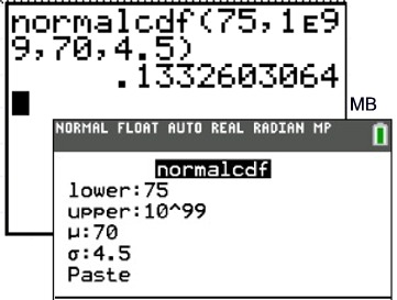
1b: Find the probability that a value is greater than or equal to
75.
(The upper boundary
in this problem will be positive infinity. The largest
value the calculator can handle is 1 x 1099
.
Type 10^99 to represent postive infinity, [or type 1 EE 99. Enter the EE by pressing 2nd,
comma -- only one E will show on the screen.]
Answer: The
probability is 13.326%.
|
|
|
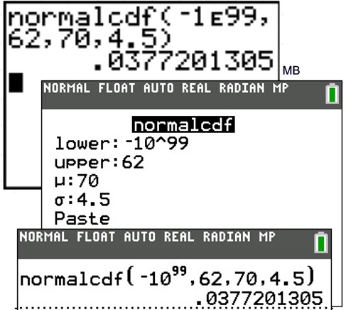
1c:
Find the probability that a value is less than 62.
(The lower boundary in this problem will be negative
infinity. The smallest value the calculator can handle is -1 x
1099
Type -10 ^ 99 [or type -1 EE 99. Enter the EE by pressing 2nd, comma -- only one E will show on the screen.]
Answer: The
probability is 3.772%.
|
|
|
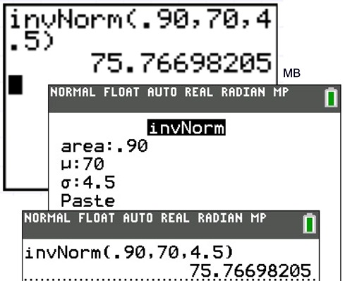
1d: Find the 90th percentile for this distribution.
(Given a probability region to the left of a value (i.e., a
percentile), determine the value using invNorm.)
Answer: The x-value is 75.767.
|
|
Example 2:
Graph and investigate the normal
distribution curve where the mean is 0 and the standard
deviation is 1. |
|
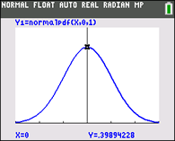
For graphing the normal distribution,
choose normalpdf.
The normalpdf (normal probability density function) is found under
DISTR (2nd
VARS) #1normalpdf(. |
|
|
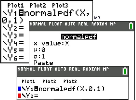
Go
to the Y = menu.
The
parameters will be (variable, mean, standard deviation).
|
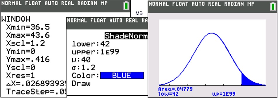
Adjust the WINDOW.
You will have to set your own window.
Guideline
is:
Xmin = mean - 3 SD
Xmax = mean +
3 SD
Xscl = SD
Ymin = 0
Ymax = 1/(2
SD)
Yscl = 0 |
|
GRAPH. Using TRACE, simply type the desired x value
and the point will be plotted.
 |
| Investigate: What
happens to the curve as the standard deviation increases? |
Double the standard deviation
and see what happens to
the graph.
|
When graphing 2 normal curves, the window will need to be adjusted.
|
Xmin = mean - 3 (largest SD)
Xmax = mean +
3 (largest SD)
Xscl =
largest SD
Ymin = 0
Ymax = 1/(2
smallest SD)
Yscl = 0 |
|
Observe that as the standard
deviation increases, the more
spread out the graph becomes. |
|
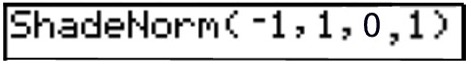
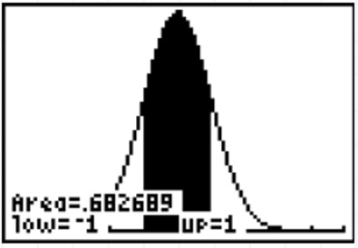
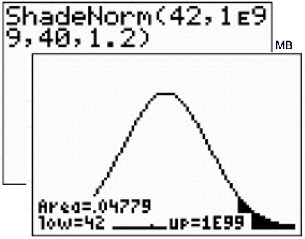
Now, the area under the curve between particular values
represents the probabilities of events occurring within that
specific range. This area can be seen using the
command ShadeNorm(.
Before attempting ShadeNorm, be sure that
Y1 = normalpdf(x, mean, standard deviation) is active and that the appropriate window has been set as indicated in the Window Guidelines in the previous section.
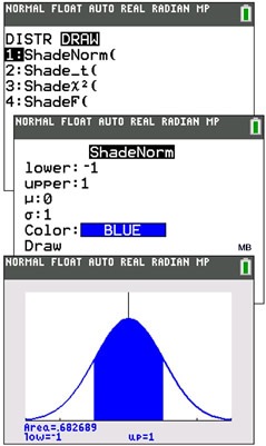
To find ShadeNorm(,
go to DISTR
and right arrow to DRAW.
Choose #1:ShadeNorm(.
ShadeNorm (lower bound, upperbound, mean,
standard deviation)
Notice that the calculator defaults to a mean of 0 and a standard deviation of 1 unless changed by the user. Remember that there is approximately a 68% probability of a score falling within 1
standard deviation from the mean in a normally distributed
set of values. The "area" value in this graph is indicating 0.682689 or approximately 68%.
  |
|
| Notice how this answer supports the
percentage listed in the chart at the top of this page. |
| Example 3: Graph and examine a
situation where the mean score is 46 and the standard
deviation is 8.5 for a normally distributed set of
data. |
|
|
Go to Y= .
|
Adjust the window. |
GRAPH.
 |
|
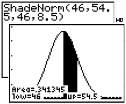
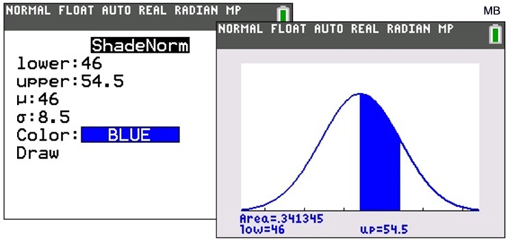
Examine: What is the probability of a value falling
between the mean and the first standard deviation to the
right? Answer: approximately 34%
Notice how this percentage supports the
information found in the chart at the top of this page for
the percentage of information falling within one standard
deviation above the mean.
|
|

 ShadeNorm( go to DISTR and right arrow to DRAW.
Choose #1:ShadeNorm(.
ShadeNorm( go to DISTR and right arrow to DRAW.
Choose #1:ShadeNorm(.